INTRODUCTION

All matter contained in water – except for solute – is collectively referred to as solids [18]. These contain rock components of various origin, density, grain size and shape. The solids are subdivided according to the mode of their transportation. Generally one can recognize two types of sediments in rivers: bed load and suspended load. In mountain stream where the streambed consists mostly of gravel and coarse sands bedload is reported to constitute c.a. 70 per cent of total bedload [28], whereas for some large rivers it is even less then 1 per cent. While moving, rolling, skipping or sliding downstream along the river bottom the bedload tends to produce sediment structures attached to a riverbed or to its banks. Such structures are commonly recognized as channel bars.

River bars, or closely related features, are typical for all rivers and are mimicked in the other linear shear flows [7]. So far, no formal criterion has been developed for occurrence of bars in terms of flow and sediment characteristics. Bars, defined as accumulation of sediment grains, or sand and/or gravel deposits [28], cannot develop if the flow depth is approximately equal to the minimum grain size [7]. Considering alluvial channel three types of bars could be commonly recognized: alternating bars, point bars and braid bars [28]. Alternating bars form in straight channels segments within curves of meandering thawleg. Point bars develop in the areas of relatively low stream power at the inside of channel meander. Braid bars, mostly diamond-shaped, are often associated with coarse material (Figure 1). They are aligned to the flow and called longitudinal bars [28]. Although bar forms have been commonly described in sandy or gravely meandering rivers, little attention has been given to the role of obstructions in controlling geomorphic forms in coarse-grained environments [3,5,10]. As far as geometry of a mountain stream is concerned bars start to develop in its middle and lower reaches where the channel reaches high width to depth ratios [2]. Deposition of river bar is directly related to bend curvature reflecting especially a role of sharp bands in arresting sediment under lower energy conditions. Other reasons for bar depositions are obstructions or hindrances caused by large boulders or bedrocks (this is a common spot where re-attachment bars are formed), or wooden logs behind which sediment is trapped. Some basic shapes of gravel bars are presented (Figure 2).

Figure 1. Gravel river bars shapes

Figure 2. Typical gravel river bars

There are only a few studies on the role bars play in gravel stream environment, especially in shaping a river channel (Figure 3) and stopping bank erosion. Bars should be treated as roughness elements, equally or even more important than channel bed roughness associated with dimensions of grains forming riverbed [25]. This seems to be of a great interest especially for high floods.

Figure 3. Typical shapes of river channels

The purpose of this paper is to examine the changes of granulometry along stream bars which are formed in the different hydrodynamic conditions connected with the chanell shape. The question asked is if it is possible to develop a quite stable gravel structure sitting on a stream bed which could in a way stabilize stream channel and its banks. The second purpose of the work was to find out the differences in hydraulics conditions accompanying the regions closest to the already developed gravel bars situated in small, mountain stream. The stream of interest is in the area of the Polish part of The Carpathian Mountains close to the Babiogórski National Park. Finally, the chemistry of sediments depisited within the bars and their regions was examined.

STUDY AREA

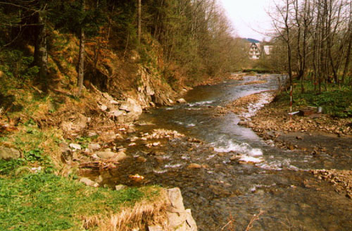
The upper part of the Skawica-Jałowiecki Stream in the Polish part of The Carpathian Mountains (Figure 4) is situated in the Carpathian flysh. The stream is flashy and experiences frequent bed load movement. Its streambed consists mostly of sandstone and mudstone bed-load pebbles and cobbles forming a framework, the interstices of which are filled by a matrix of finer sediment.

Figure 4 a, b. Catchment study region with the detailed sketch of the research reach

Table 1. Physical characteristics of sites investigated

Variables	Skawica-Jałowiecki
Precipitation [mm] Catchment Area [km2] Channel gradient [-] Max. Stream width [m] Max. Stream depth [m] Mean annual discharge [m3 s-1] Two years flood Q50% [m3 s-1] Ten years flood Q10% [m3 s-1] Bank full [m3 s-1]	1189 19.33  0.085  16.3  0.83  1.39  12.6  48.8  32.0 – 40.0

Suspended sediment loads are small and contribute insignificantly to channel morphology. Within the 1109.5 m long studied reach Skawica-Jałowiecki cuts through an alluvial bed, mostly Quaternary, Holocene river gravels, sands and mudstones [15]. Upstream-investigated reach just borders upon a Tertiary, Palaeogene reach where mica-sandstone, sandstone, mudstone and phyllite predominate.

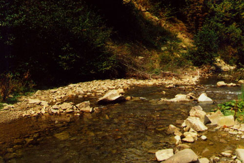
Many gravel river bed-forms, such as point and middle bars, can be noticed within investigated Skawica-Jalowiecki reach. Most gravel bed-forms growing behind and in front of obstacles (Phot. 2), especially those situated at riverbanks (meander-bars) are durable (Phot. 1). The detailed geology and geomorphology of the region has been described in Radecki-Pawlik [26]. Some basic physical characteristics of the catchment study area are presented in Table 1.

METHODS

For the purpose of this study the 1109.5 meters long research reach (Figure 4) was found within Zawoja municipality. Identification and field measurements of bed forms were carried out during the Summer of ‘98 and the early Spring of 2000. The study one can divide in two parts: first was based on a detailed granulometric study of chosen gravel bars (Figure 5); second: on a hydraulics survey of the water velocity close to the streambed within research cross sections to calculate shear stresses, drag coefficients and other hydraulics characteristics. Also in that region there were sediment samples taken directly from the stream bed.

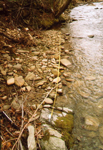
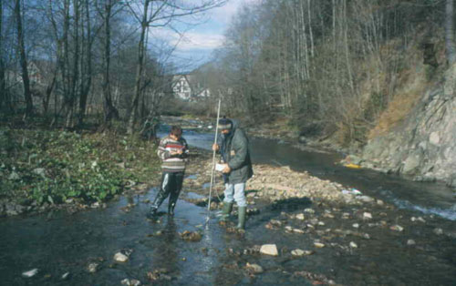
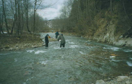
Two well-developed streambed features were recognised as point bar “a” situated downstream of a stream band (Phot. 1)at the upper part of the reach and an upstream of obstruction bar (the obstruction in that case was a radiolarite megacluster) attached to the right bank of the creek – alternation bar “b” (Phot. 3). Within the region of investigated bars research cross section were established and within them measuring points were fixed. In all of those points wading velocity measurements were performed (Figure 6, Phot. 4, 5, 6).

Figure 5. Cross-section of investigated granulometry and within the point bars “a” and “b”. Also the points of sediment-chemical samples are marked.

Figure 6. Investigated gravel bars “a” and “b” with velocity measuring points

Photo 1. Meander-like point gravel bar partly excavated after a spring flood

Photo 2. Up-stream of obstruction alternate gravel bar. The obstruction in this case is a middle log jam

Photo 3. Up-stream of obstruction alternate gravel bar. The obstruction in this case is a megacluster

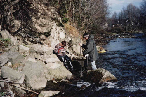
Photo 4. Wadding measurements within gravel point bar region under low discharge

Photo 5. Wadding measurements within gravel point bar region under annual flow discharge

Photo 6. Wadding measurements in a shadow of megacluster where fine sediment is deposited

For 30.25 m long point bar “a” 11 (Figure 5, Phot. 3) cross-survey sections were examined and gravel samples were taken from each. Similarly, for 11.25 m long side bar “b” the data for sieving analysis were collected in 7 cross sections. Since the sediment deposited on two bars consists basically of two layers, surface and subsurface, the technique of sampling described by Church, McLean and Wolcot [8] was applied. The bar surface layer was identified rather as armoured than censored and definitely not paved [3, 21]. Because the bed surface material is the focus of interest in flow resistance, competence investigation and classical studies of surface coarsening [8], subsurface material from bars “a” and “b” was collected after clearing the surface to the depth of the deepest-lying exposed grain on the bars. Samples were collected from homogeneous body of sediment, so as not to combine them with the distinct surface material. Next, the sieving analys is for coarse grains was carried out then in the field using round-mesh sieves for hand work [20]. Fine material was carefully collected and analysed in a laboratory.

Below are listed the grain field characteristics of collected materials [9]. All the coefficients and indicators were calculated for the two point bars “a” and “b” in all surveyed cross sections of the bars:

- the Trask sorting coefficient

- Hazen’s sorting coefficient

- Knoroz’s grain-size diversity indicator

- Kollis' uniformity indicator

where: d₅, d₁₀, ...d_i – characteristic grain-size diameters of river bed in metric units.

Grain-size parameters commonly used by geomorphologists [12,18] are as follows:

- inclusive graphics standard deviation after Folk:

- mean value after Folk

skewness coefficient

- curtosis

where: φ₅, φ₁₆, ...φ_i - characteristic grain-size diameters of river bed in “phi” units.

Water velocity measurements were based on Jarrett’s [14] findings regarding the taking of velocity profiles in mountain stream cross-sections (Figure 6). Gordon and others [11] and Bergeron and Abraham’s [1] methods were then applied to the field data, and shear velocity V_* values were calculated from the velocity profiles obtained near-to-river-bed. Finally, shear stress t values were calculated from:

where: r - water density [kg m^-3] and V_* - shear velocity [m s ^-1].

Shear stress value (V_*) is obtained just directly from the equation v = f (D) [11]:

V_* = a / 5.75

where: a – slope coefficient of v = f (D),
according to the general line equation: v = aD + b,
where: D – water depth above the stream bed [m], b – constant.

To calculate the flow resistance coefficient (f) the comments given by Ven Te Chow [6], Wijbenga [30] and Przedwojski et al. [23] were used. Flow resistance coefficient was obtained from:

f = 8 (V_*/ V_¶r)²

The detailed way of obtaining of all above mention parameters using classic hydraulics equations are shown in Radecki-Pawlik [26]. Bed-load sediment deposited in the area, where hydraulics data were measured was also collected. Here the technique of sampling described by Wolman [31] was applied. Later, grain size curves were plotted and characteristic grain dimensions were read. Additionally, for grain shape analysis 339 single grains were chosen randomly from the riverbed and carefully measured. Grain shapes were described according to Zingg [11,12]. Bankfull was calculated using various equations presented in other authors paper [27], whereas t-years floods were found according to Punzet equations [24]. The chemistry of sediments was examined using the methods as follows [13]:

- mechanical components of sediments: using Casagrande’a metchod in Prószyński modification,
- pH in H₂O and in KCl: using a potentiometry method,
- specific weight: using a pycnometer method,
- organic matter: using an annealing method,
- Mg, K, Ca, Cr, Mn, Fe, Ni, Cu, Zn, Cd, Pb: using 8200 Hitachi spectro-photometer,
- C: using Tiurina’e method,
- Na: using Kiejdahla’e method,
- S: using Butters-Chenery method.

RESULTS

All results obtained are presented in tables for the paper clarity reasons. All basic granulometric parameters calculated for each of the researched bars and recognized by geomorphologists are jointly presented in tables 2, 3, 4 and 5. Table 2 and 3 show all characteristic grain sizes, which are used for sedimentological calculations and bedload transport calculations. Sediment indicators and characteristics are given in tables 4 and 5. Thus, the Table 6 and 7 show all hydraulics parameters measured and calculated above research points within the region of investigated bars (Figure 3). Wadding measurements were taken under two discharges. The first was Q=0.34 m³/s which is close to the mean annual flow (Q=0.46 m³/s ) - Table 1, whereas the second discharge was a spring flood when Q reached 1.04 m³/s. Under the second discharge conditions the bed load movement was noticed. The sediment samples were taken from all the places where the velocity measurements were done, right after the water dropped. Sediment data are presented in the form of characteristic grain dimensions – Table 8, 9 – and as shape dominant grains – Table 10.

Table 2. Basic sediment grain-size dimensions – point bar “a”

	Cross sections
	a1-a1	a2-a2	a3-a3	a4-a4	a5-a5	a5-a6	a7-a7	a8-a8	a9-a9	a10-a10	a11-a11
d5 =	1.07	0.36	1.13	0.6	0.83	0.5	0.84	0.92	0.82	0.8	0.54
d10 =	3.76	0.92	2.48	1.37	1.53	1.0	1.61	1.26	1.6	1.6	1.14
d16 =	6.9	1.7	4.5	2.83	2.93	1.66	3.62	2.47	3.74	3.76	2.36
d25 =	12.26	4.11	8.37	5.47	5.76	4.18	8.24	6.07	7.75	7.87	6.0
d50 =	27.5	18.46	26.45	16.26	21.07	22.7	27.36	19.7	22.84	20.88	20.26
d60 =	35.46	24.98	42.04	22.9	26.91	30,0	43.09	27.16	28.66	28.42	27.37
d75 =	49.35	41.68	70.24	34.72	38.43	53.41	90.3	41.03	39.84	41.73	44.21
d84 =	68.0	57.0	91.7	44.6	46.3	71.4	111.8	50.0	46.8	49.9	64.7
d90 =	90.26	68.15	106.09	52.5	71.18	76.52	126.12	59.75	54.32	62.42	86.8
d95 =	110.13	98.89	118.05	63.86	100.59	80.76	138.06	68.02	65.68	74.37	105.9

Table 3. Basic sedimentological parameters – point bar “a”

	Cross sections
	a1-a1	a2-a2	a3-a3	a4-a4	a5-a5	a6-a6	a7-a7	a8-a8	a9-a9	a10-a10	a11-a11
GSS	-5.363	-4.403	-5.17	-4.327	-4.423	-4.29	-5.133	-4.387	-4.587	-4.587	-4.6
GSO	1.75	2.37	1.97	1.9	1.94	2.1	2.31	2.00	1.76	1.77	2.3
GSK	-0.181	0.093	-0.196	0.096	0.06	0.174	-0.126	0.107	0.094	0.054	0.01
GSP	1.65	1.055	0.818	1.005	1.05	0.885	0.836	1.061	1.24	1.208	1.148
S0	2.01	3.18	2.9	2.52	2.58	3.57	3.31	2.6	2.27	2.3	2.71
u	9.43	27.15	16.95	16.72	17.59	30.00	26.76	21.56	17.91	17.76	24.01
e	102.93	274.69	104.47	106.43	121.19	161.52	164.36	73.93	80.1	92.96	196.11
Cd	0.45	0.18	0.38	0.27	0.25	0.15	0.27	0.19	0.17	0.23	0.24

Table 4. Basic sediment grain-size dimensions – upstream of obstruction bar “b”

	Cross sections
	b1-b1	b2-b2	b3-b3	b4-b4	b5-b5	b6-b6	b7-b7
d5 =	0.23	0.25	1.36	0.29	0.32	44.81	32.47
d10 =	0.37	0.44	6.23	0.78	3.67	54.5	47.33
d16 =	0.6	0.7	14.4	4.7	12.0	60.7	53.4
d25 =	1.69	6.71	37.1	17.59	22.8	70.0	59.28
d50 =	17.3	26.31	71.48	73.87	50.27	90.11	75.93
d60 =	23.68	41.16	80.18	82.09	64.16	98.08	82.74
d75 =	73.18	79.05	93.24	94.43	78.93	110.05	92.96
d84 =	90.0	86.6	101.1	101.8	86.5	117.2	99.1
d90 =	101.27	91.62	106.29	106.77	91.57	122.02	103.18
d95 =	110.64	95.81	110.65	110.89	95.79	126.01	106.59

Table 5. Basic sedimentological parameters – upstream of obstruction bar “b”

	Cross sections
	b1-b1	b2-b2	b3-b3	b4-b4	b5-b5	b6-b6	b7-b7
GSS	-3.96	-4.34	-6.24	-5.63	-5.79	-7.05	-6.69
GSO	2.82	2.68	1.45	2.24	1.71	0.43	0.39
GSK	0.20	0.25	0.23	0.47	0.21	-1.86	-2.12
GSP	0.745	1.063	1.936	1.639	2.158	1.863	0.939
S0	6.58	3.43	1.59	2.32	1.86	1.25	1.25
u	64.00	93.55	12.87	105.2	17.48	1.80	1.75
e	481.0	383.2	81.4	382.4	299.3	2.8	3.3
Cd	0.13	0.06	0.13	0.02	0.13	0.82	0.85

Table 6. Results of hydraulic measurements and calculations – point bar “a”

Point number	Water discharge Q [ m3 · s-1]	Froude number (Fr)	Shear velocity (V*) [cm · s-1]	Reynolds number (Re)	Shear stress (t) [N · m-2]	Flow resistance coefficient (f)
1A	0.34	0.20	1.95	7 571	0.38	0.1225
1B	0.34	0.30	8.59	488 851	7.39	0.4367
1C	0.34	0.20	4.11	16 886	1.69	0.3021
2A	0.34	0.30	8.39	10 6663	7.06	0.9053
2B	0.34	1.50	11.98	10 6555	14.36	0.0543
2C	0.34	0.08	1.50	15196	0.25	0.1466
3	0.34	0.44	4.48	38 862	2.01	0.0787
4	0.34	0.10	5.23	16 282	2.74	0.8835
1A	1.04	0.60	79.61	94 623	22.30	0.2823
1B	1.04	0.70	15.50	182 856	24.00	0.1414
1C	1.04	0.40	8.87	43 015	7.80	0.2885
2A	1.04	1.06	17.60	221 360	31.10	0.1015
2B	1.04	0.50	11.09	57 007	12.30	0.3239
2C	1.04	0.01	0.19	1 637	0.01	0.3136
3	1.04	0.80	31.77	211 493	100.93	0.0444
4	1.04	0.80	11.41	75 261	13.04	0.1555

Table 7. Results of hydraulic measurements and calculations: up-stream-of-obstruction bar “b”

Point number	Water discharge Q [m3 · s-1]	Froude number (Fr)	Shear velocity (V*) [cm · s-1]	Reynolds number (Re)	Shear stress (t) [N · m-2]	Flow resistance coefficient (f)
1A	0.34	0.43	2.50	48 358	0.62	0.0205
1B	0.34	0.50	8.37	42 930	7.02	0.2255
1C	0.34	0.40	3.29	30 429	1.09	0.0505
2A	0.34	0.05	1.44	9 402	0.21	0.3765
2B	0.34	0.30	7.39	67 310	5.47	0.6687
2C	0.34	0.20	5.21	18 539	2.72	0.4038
4	0.34	0.04	0.56	2 341	0.04	0.2439
1A	1.04	0.53	6.49	53 784	4.21	0.0989
1B	1.04	0.60	17.27	214 292	29.80	0.1898
1C	1.04	0.60	19.29	136 091	37.20	0.3584
2A	1.04	0.08	2.69	9 056	0.87	0.9142
2B	1.04	0.90	13.38	195 812	17.90	0.0789
2C	1.04	0.54	5.63	159 169	3.10	0.0291
4	1.04	0.50	10.93	62 525	11.90	0.2891

Table 8, 9. Characteristic grain size dimensions within the region close to investigated point bars

alternate bar “b”
	d5	d10	d16	d25	d50	d60	d75	d84	d90	d95
1A	77.6	95.4	115.7	146.2	230.8	264.6	315.4	345.9	366.2	383.1
1B	14.8	25	39.6	55.3	72.3	74.5	77.8	79.8	109.5	138.7
1C	6.1	10.8	15.3	20.6	36.2	42.9	52.1	56.4	59.2	76.1
2A	15	28.5	34.9	42.9	73.2	96.6	131.6	152.6	166.7	178.3
2B	21.1	32.6	43.8	54.4	72.8	78.6	133.3	171.7	197.3	218.7
2C	7.8	13.5	19.8	29.2	45.4	52	76.2	111.8	135.5	155.2
4	22.1	33	46.9	70.8	75.4	77.3	80.6	120	146.2	168.1
point bar “a”
1A	18.5	34.1	54.4	70.4	77.5	82.2	111.4	128.9	140.6	150.3
1B	41.2	70.2	71.1	72.5	76.4	77.9	90.1	151.2	192	226
1C	20.3	32	43.2	56.5	74.4	77.6	107.8	141	163.1	181.6
2A	15.8	25.5	36.4	52.6	74.7	77.5	105.7	143.3	168.3	189.1
2B	14.3	17.9	21.7	27.4	45.2	51.3	56.8	61	98.1	129.1
2C	0.002	0.003	0.01	0.02	0.13	0.21	0.34	0.41	0.47	0.51
3	11.1	18.9	28.9	49.3	94.3	117.4	152.1	173	186.6	198.4
4	24.6	37.9	50.4	60.9	76.3	80	136.2	170	192.5	211.2

Table 10. Percentage of different grain shapes of  bed load

Grain shape	Percentage
Spherical	4.43
Bladed	41
Disc-shaped and rod-like	54.57
100 %

Table 11. Chemical properties of alluvial sediments in the Skawica-Jałowiecki Stream

Sample No Component	ZI-1 point bar b	ZI-2 point bar b	ZI-3 point bar b	ZIV-1 point bar a	ZIV-2 point bar a	ZIV-3 point bar a	ZIV-4 shadow of the rock	back- ground (flood plain)
Spec. weight [g/cm3]	2.69	2.68	2.63	2.7	2.72	2.67	2.62	2.69
Organic material [%]	3.15	3.12	3.43	3.61	3.50	3.81	3.86	3.62
Cr [ppm]	62.4	47.5	69.7	64.4	65.7	44.8	64.4	73.7
Mn [ppm]	33.5	34.3	32.4	34.3	39.1	42.6	29.4	41.0
Fe [ppm]	27094	27310	27684	30814	30475	30335	23777	22131
Ni [ppm]	66.4	66.2	70.0	51.2	78.9	79.3	77.8	70.9
Cu [ppm]	32.9	22.5	23.8	28.3	23.8	24.9	19.5	17.7
Zn [ppm]	73.9	68.9	74.4	71.6	75.0	79.6	71.7	65.8
Sr [ppm]	10.7	13.1	13.1	11.8	12.3	16.5	10.7	7.3
Cd [ppm]	0.20	0.25	0.1	0.15	0.1	0.45	1.3	0.55
Pb [ppm]	14.5	12.5	16.2	16.7	13.9	15.3	33.2	83.9
j 1-0.1 [mm]	69	77	70	58	79	80	56	37
j 0.1-0.05 [mm]	8	6	6	12	2	4	13	22
j 0.05-0.02 [mm]	4	5	7	10	5	2	12	15
j 0.02-0.005 [mm]	8	6	6	6	8	8	7	8
j 0.005-0.002 [mm]	5	3	7	10	4	4	8	9
j < 0.002 [mm]	6	3	4	4	2	2	4	9
C [%]	0.72	0.36	0.3	0.48	1.02	0.42	0.72	0.48
N [%]	0.029	0.027	0.032	0.045	0.034	0.042	0.067	0.087
S [%]	0.051	0.042	0.075	0.071	0.044	0.055	0.066	0.023
pH in H2O	7.9	8.0	8.1	7.5	8.0	8.0	6.6	6.6
pH in KCl	7.2	7.1	7.2	7.1	7.2	7.2	6.8	5.6
Conductance [µS/cm]	0.1	0.1	0.1	0.45	0.14	0.14	0.11	0.07

It is also important to mention geodesical survey in point bar “a” and “b” region carried out simultaneously with sediment analysis. Extremely detailed survey revealed that during the observation period between August 1998 and April 2000 a denivelation of the “a” bar was changed 0.5 prommill (it was 18.3 prommill in August 1998 and dropped down to 17.8 prommill in April 2000). Also a slight denivelation in cross-section profile within the bar “b” region was detected where the left bank was undercut a little and slumped into the river channel. As a result, a thalweg was shifted towards a concave bank and close to the a3-a3 cross section a small pool started to develop. Cross-sections a1-a1 and a2-a2 moved slightly downstream, whereas a cross-section a4-a4 was build-up. At the same time cross-sections from a5-a5 to a9-a9 were slightly washed out and the bar in that region grew wider. Finally, cross-sections a10-a10 and a11-a11 were again built up, accommodating more sediment. It was reported by the land survey that the whole structure ”a” moved downwards around 2 meters.

When analysing geodesical survey data for the “b” bar structure, one could observe a rise in its slope from 14.2 prommill in August 1998 to 15.9 prommill in April 2000. Close to the middle part of the structure “b” the stream channel was degradated by c.a. 0.07m and the thalweg moved towards the left bank. The bar length was slightly cut 0.3 m. In sections b2-b2, b4-b4 and b7-b7 the riverbank at the point bar was undercut a little. At the same time in sections b3-b3 and b4-b4 the structure was built up whereas in the cross section b5-b5 the bar widened a little.

DISCUSSION

Before discussing the sediment structure of the both bars described in the paper it seems quite important to mention the existence of many form roughnesses, which were recognised within the study region. Such form roughnesses are commonly recognised in all mountain streams [10] and have to be considered within a hierarchy of bed forms – for example clusters are superimposed on bars, complex clusters form part of cobble berms, megaclusters are often components of log-jams etc. Within the “a” bar region some form roughnesses were detected, like: imbricate clusters, multiple obstacle clusters and many two-particle clusters. Also, just after spring flooding a single string of large clasts sitting approximately normal to the streamline appeared on the bar “a”. Carling and Komar [4] explains that such clasts (>200mm) once make contact with each other the likelihood of any one particle being moved a significant distance from its neighbours is low. Within the region of bar “b” one could recogniz e such form roughness as two particle clusters, multiple obstacle clusters and complex clusters. Also Ostler lenses [19] formed on the downstream part of boulders, attached to the inner, proximal part of the bars were detected. It has to be remembered that many of form roughnesses are swept away during flooding, thus only few of them are durable.

Referring to all granulometric parameters calculated from sedimentological samples for point bar “a” one could see that inclusive standard deviation value varies here from 1.75 to 2.37, coefficient of sorting changes from 2.01 to 3.57, Hazen’s sorting coefficient varies from 9.43 to 30, Knoroze’s grain size diversity is between 80 and 274.7 and finally Kollise’s uniformity indicator is between 0.15 and 0.38. All those results show that the mentioned point bar “a” is poorly sorted (GSO=1.0 – 2.0) and very poorly sorted (GSO=2.0 – 40.0) along its body. GSK value is from 0.26 to 0.57, GSP (curtosis) is from 0.818 up to 1.650 and finally d₅₀ varies from 18.5 – 27.4 mm, which means that the bar is quite the same along all the structure. Thus, the point bar “a” structure could be assessed as a young structure, poorly sorted, not durable and poorly developed. It leads to a conclusion that point bars, prone to changes during floods develop at the stream band and such changes are noticeab le within nearly one hydrological year.

A different situation was noticed along the upstream of the obstruction bar “b”. Here GSO varies from 2.82 – 2.24 at the proximal part of the structure (poorly sorted) to 0.43 – 0.39 (well sorted) at the distal part of the structure. The same goes with Track’s S_o (sorting coefficient) which drops from 6.58 (tail part of the structure) down to 1.25 value – just behind the obstacle. Hazen’s sorting coefficient varies from 64 to 1.75, Knoroz’s grain size diversity parameters drop from 484 to 3.82 at the distal part of the bar “b”. At the same time d₅₀ decreases from 90.1 to 17.3 mm, which means that grain sizes are getting larger at the distal part of the “b”. With such results it seems quite clear that we have here a well-developed and durable gravel streambed feature quite resistant to floods. The bar “b” is not the same as far as its texture is concerned. In the distal part of it there is hardly any fine sediment to be noticed whereas the coarse sediment predominates. Going to the proximal part of the feature it is evident that fine sediment predominates here. Probably the obstacle behind which the bar “b” formed shadows coarse particles, which are hidden here and immobilised even during flooding. On the other hand fine particles are winnowed from here even during low floods and if they are accommodated they are sitting at the proximal part of the structure, which for that reason is prone to changes (this part of the bar “b” was cut about 30 cm within a period of few month when this study was carried out). But one had to notice that as the whole the structure is quite stable. Moreover, the riverbank along the bar “b” is also stable. It seems that such gravel formation like the upstream of the obstruction bar “b” acts as a natural riverbank protection, which is often constructed by men and called longitudinal dike. In other words it protects a riverbank against erosion.

The sediment deposited within the region of investigated bars (Figure 6) varies in diameters along the structures as well as across the cross sections of the stream. In general, d₅₀ is between 36.2 – 230.8 mm (a representative grain size), d₁₆ is between 15.3 – 125.7 mm and d₈₄ between 56.4 – 345.0 mm. The biggest differences in sediment diameters were noticed along alternate bar “b”. Along point bar “a” the coarser sediment deposited very close to the bar structure – point 3 – where also the highest value of shear stresses t =100.93 N/ m² was noticed as well as shear velocity (all calculated for Q=1.04 m³/s flood discharge). Above point 2B the biggest shear stress value t = 14.36 N/ m² were found under the mean annual flow (Q=0.34 m³/s). Under this conditions Fr was >> 1, whereas at 2B under Q=1.04 m^{3/s Fr was < 1 and shear stresses and shear velocity were significantly smaller here then under mean annual flow conditions. It seems the water here behaves like above a typical riffle in the riffle and pool sequence when reversal velocity phenomena could be noticed. Point 2C is an extraordinary one since it lies in the shadow of the rock piled up on the streambed. The fine sediment here is deposited in a huge amount and even under flood conditions Fr is still << 1.}

Along alternate bar “b” the coarser sediment deposited in 1A and 4 points, again close to the bar structure. The highest values of shear stresses under flooding conditions are above 1B and 1c points. The biggest shear stress value under annual discharge is again in 2B point. The finest sediment is deposited along the left bank of the stream – opposite to the developed alternate bar structure. Point 2A is in the shadow of the bar. Shear stresses and shear velocity are the smallest here. The thawleg line, in the contest of hydraulics parameters, seems to work like a vertical riffle of the reach. Along that line Fr, shear stresses and shear velocity are the biggest under both run discharges.

According to Lityńskiego et al [17] pH in KCl for all sediments samples is above 7.0 (from 7.0 to 7.2), which means all samples are basic. At the same time pH from back-ground (which in the case of the study is the floodplain) (ZIII-4) is slightly acidic (still close to inactive). The same goes (a slightly acid pH) with the sample taken from the place which is situated in the shadow of a very large rock, under the water, where fine sediment predominates (d<2mm) across the point bar “a”. For all collected samples conductance value is relatively low. As far as heavy metals are concerned, the biggest value of Pb=83.9 ppm one can notice in the floodplain sample, which is close to maximum value according to PIO¦ [22]. The same situation is with Cd =0.55 ppm. In the floodplain sample is proportionally small amount of Cu when comparing it with samples taken from the bars. In all samples Cr amount is bigger then critical according to Lis and Pasieczna [16], as well as Cu amount. In ZIV-1 sampl e the conductance is 3 times bigger then in other places. The bigger amount of Pb=33.4 and Cd=1.3 was found in the fine sediment situated in the shadow of the rock in front of the point bar a”. In samples taken from the point bar “b” the biggest amount of Cu=32.9 is in ZI-1 (at the shadow of the bar “b” where there is the finest sediment).

CONCLUSIONS

The analysis of hydraulics and sediment results within the region of investigated bars leads to the following conclusions:

1. There are many different streambed forms and form roughnesses which develop in mountain stream. Some of them are much more stable and durable then others. Closer attention paid to and careful studies of such bed forms are necessary as they have a huge influence on bank channels and channel bed stabilisation.

2. It is possible to develop quite stable river bar in the mountain stream channel. Such structure seems to be the alternate bar, developed up-stream of the obstacle. Its existence could have a huge influence on stopping a stream bank erosion as well as stabilize a stream bed.

3. If a developed stream bar is stable it protects a channel bank against erosion and under-cutting in the same way as some artificial longitudinal dikes constructed for river training reasons.

4. The coarser sediment in the cross section is deposited along the outer line of developed bars. That way bars are in a constant process of up building. Especially the distal part of the bars is quite stable.

5. The finest sediment is deposited at the opposite bank to where the bars are formed. The shear stresses, Fr and shear velocity values are the smallest here.

6. There are some places within the stream reaches called “shadows” where the finest sediment is deposited even under flooding. Such shadows could be find behind rocks and/or proximal part of bars.

7. For the alternate bars “b”- the highest values of shear stresses, shear velocity and Froude number are along the thawleg line lying approximately in the middle of the stream cross sections within a bar region.

8. For the point bar “a”– the highest Froude number is noticed in the proximal part of the bar, at the entrance between the bar and the opposite bank, along the thawleg. Under annual flow conditions it is possible to find places within a region of point bar working like riffle and pool sequences, when reversal velocity phenomena could be notice.

9. As the shapes of grains deposit in the mountain, alluvial stream, the highest percentage of them are disc-shaped and rod-like. The next ones are bladed. The spherical grains are just a small percentage of all (less than 5%).

10. Heavy metals such as Cd, Pb and Cu are likely to accommodate in fine sediments deposited in the stream and/or in stream bars, especially in shadows of big rocks but also in shadows of well-developed point bars. Their presence is associated though with the grain size of sediment but also with bars durability.

ACKNOWLEDGEMENTS

The author would like to thank graduated students of The Jagiellonian University in Krakow, Agricultural University in Krakow and Technical University of Krakow involved in the fieldwork: Radosław Radoń, Janusz Latoń, Katarzyna Przybyła, Patrycja Zasępa, Tomasz Tekielak and Bartosz Radecki-Pawlik. They were often working long hours, sieving tones of gravel and staying in cold water in a changeable weather with the never-ending enthusiasm. Great thanks to Natalia Florencka (MSc) from AGH University in Cracow for her help with chemical analysis and technical literature she provided. Finally thanks to Janet Tomkins from the Vancouver Public Library in British Columbia in Canada for her language assistance and kind corrections.

REFERENCES

1. Bergeron, N. E., Abrahams, A. D.; 1992. Estimating shear velocity and roughness length from velocity profiles. Wat. Resour. Res., 28 (8), p. 2155-2158.

2. Chang H.H.; 1980, Geometry of gravel stream, Journal of Hydraulics Div, ASCE, 106, 1443-1456.

3. Carling P.A., Reader N.A.; 1981. Structure, composition and bulk properties of upland stream gravels. Earth Surface Proc. and Landforms, vol.7, p. 349-365.

4. Carling P. A., Komar P. D.; 1991, Grain sorting in gravel – bed streams and the choice of particle sizes for flow-competence evaluations. Sedimentology 38, 498 – 502.

5. Carling P. A., Glaister M. S.; 1987. Rapid deposition of sand and gravel mixtures downstream of a negative step: the role of matrix-infilling and particle-overpassing in the process of bar-front accretion. Journal of the Geological Society, London, Vol. 144, 543 – 551.

6. Chow, Ven Te; 1959. Open-Channel hydraulics. McGraww-Hill, New York, p.108-114.

7. Church M.A., Jones D.; 1982. Channel Bars in Gravel-Bed Rivers, Gravel-bed Rivers, Edited by R.D.Hey, London, p.291-325.

8. Church M.A., McLean J.F. and Wolcot J.F.; 1987. River Bed Gravels: Sampling and Analysis. In Sediment Transport in Gravel-bed Rivers, Edited by Throne C.R. et al., John Wiley and Sons Ltd, London, 43-87.

9. D±bkowski L., Skibiński J. and Żbikowski A.; 1982. Hydrauliczne podstawy projektów wodnomelioracyjnych [Hydraulics bases for water-reclamation projects]. PWRiL, Warszawa, pp.533 [in Polish].

10. De Jong C., Ergenzinger P.; 1995. The interaction between mountain valley forms and river bed arrangement, Free University of Berlin, in River Geomorphology edited by Hickin E.J., John Wiley and Sons, New-York, p. 54-91.

11. Gordon D., McMahon T.A. and Ginlayson B.L.; 1992. Stream Hydrology. An Introduction for Ecologists. Wiley and Sons, London, pp.526.

12. Gradziński R., Kostecki A., Radomski A and Unrug R.; 1986. Zarys sedymentologii [An outline of sedimentology]. Wyd. II, Warszawa, pp.356 [in Polish].

13. Hermanowicz W., Dożańska W., Dojlido J. and Koziorowski B.; 1999. Fizyczno-chemiczne badanie wody i ¶cieków [Phisical and chemical investigations of water and sewage]. Arkady. Warszawa [in Polish].

14. Jarrett, R. D.; 1991. Wading measurements of vertical velocity profiles. Geomorphology, 4, p.243-247.

15. Ksi±żkiewicz M.; 1963. Zarys geologii Babiej Góry [An outline of the Babia Góra geology]. Zakład Geologii UJ Kraków, Materiały BPN [in Polish].

16. Lis J., Pasieczna A.; 1995. Atlas geochmemiczny Górnego ¦l±ska [Geo-chemical atlas of the Górny ¦l±sk region]. Scale 1:200000, PIG, Warszawa [in Polish].

17. Lityński T., Jurkowska H. and Gorlach E.; 1976. Analiza chemiczno-rolnicza [Agricultural and chemical analysis]. PWN, Warszawa [in Polish].

18. Mangelsdorf J., Scheurman K. and Weis F.H.; 1989. River Morphology, Springler-Verlag, Berlin-Heidelberg-New York, pp.210.

19. Martini I.P., Ostler J.; 1973. Ostler lenses: possible environmental indicators in fluvial gravels and conglomerates. J.Sedim.Petrol., 43, 418-422.

20. Michalik A.; 1990. Badania intensywno¶ci transportu rumowiska wleczonego w rzekach karpackich [Bed-load transport investigations in some Polish Carpathians rivers]. Zesz. Nauk. AR Kraków seria Rozpr. Hab., 138, pp.115 [in Polish].

21. Parker G.; 1990. Surface-based bedload transport relation for gravel rivers”, Journal of Hydraulic Research, vol. 28, 417-434.

22. PIO¦ – Environmental Protection National Agency (Państwowa Inspekcja Ochrony ¦rodowiska); 1994. Wyniki monitoringu geochemicznego osadów wodnych Polski [Geo-chemical monitoring results for the alluvial deposits in Poland]. Biblioteka Monitoringu ¦rodowiska, Warszawa [in Polish].

23. Przedwojski B., Błażejewski R. and Pilarczyk K.W.; 1995. River training techniques. Balkema, Rotterdam, Brookfield.

24. Radecki-Pawlik A. 1995. WODA-v.2.0, a simple hydrological computer model to calculate the t-year flood. In: Hydrological processes in the catchment, edited by B. Więzik, PK, Cracow, 131-141.

25. Radecki-Pawlik A.; 2002a. Okre¶lenie warto¶ci współczynnika szorstko¶ci koryta potoku górskiego na podstawie pomiarów terenowych [Field investigations of a roughness coefficient within a riffle and pool sequences of mountainous stream]. Zesz. Nauk. AR Cracow, 23, p. 251-261 [in Polish].

26. Radecki-Pawlik A.; 2002b. Wybrane zagadnienia kształtowania się form korytowych potoku górskiego i form dennych rzeki nizinnej [Some aspects of the formation of mountain stream bars and lowland river dunes]. Zesz. Nauk. AR w Cracow, seria Rozprawy, no. 281 [in Polish].

27. Radecki-Pawlik A.; 2002c. Bankfull discharge in mountain streams: theory and practice. Earth Surface Processes and Landforms, John Wiley and Sons, 27, 115-123.

28. Selby M.J.; 1985, Earth’s changing surface, Clarendon Press, Oxford, pp.607.

29. Whittow J.; 1984, Dictionary of physical geography, Penguin, London, pp.591.

30. Wijbenga J.H.; 1990. Flow resistance and bed-form dimensions for varying flow conditions. Delft Hydraulics. Part 1-4 (main text and appendix). Toegepast Onderzoek Waterstaat A58.

31. Wolman M.; 1954. A method of sampling coarse river-bed material, American Geophysics Union, vol. 35, 6, p.951-955.

Responses to this article, comments are invited and should be submitted within three months of the publication of the article. If accepted for publication, they will be published in the chapter headed ‘Discussions’ in each series and hyperlinked to the article.